This application note shows an example of user defined output data in Empire XPU.
By default, Empire creates S-parameter output files for the given port configuration. From that data, we calculate differential S-parameters. For 2-port simulation data, that is:
Zdiff = Z(1,1) – Z(1,2) – Z(2,1) + Z(2,2)
From Zdiff, we then calculate the differential impedance between the 2-ports:
Ldiff = imag(Zdiff) / omega
Defining postprocessing equations
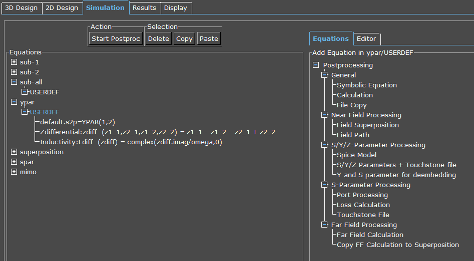
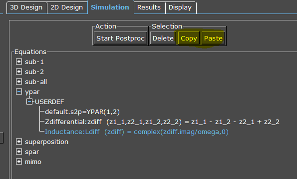
For our calulation, we need Z-parameter input data. A convenient way to create all Y+Z-param is to use output “S/Y/Z-Parameters + Touchstone file” in the ypar USERDEF section. This creates all this data in separate files in the ypar directory.
We can leave the S-parameter file name (default.s2p) and will actually use some of the other files created by this postprocessing option:
It can be seen that this postprocessing option creates all S/Y/Z parameters as individual files. We use some of this data in the next steps. Order matters for postprocessing, so it is important to place this output first, before the next steps!
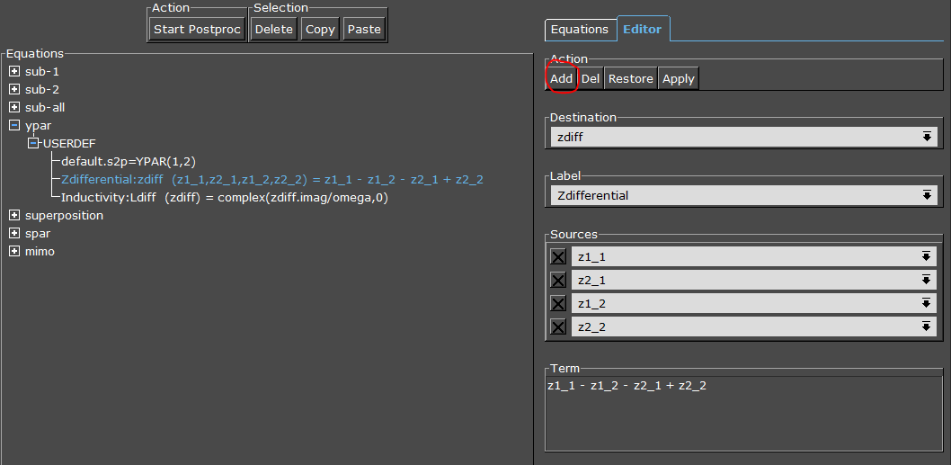
The second step is to create the differential Z from the four 2-port Z-parameters, using four input files. This is done with a “Symbolic Equation”.
For more input files, click the Add button and type the name of the file into the corresponding sources field. In our case, the complex output value is simply created by adding the complex values from the files, using the exact file names: z1_1 – z1_2 – z2_1 + z2_2. Results are written to the destination file “zdiff”.
The final step is calculate the equivalent inductance Ldiff from that differential impedance. This requires another “Symbolic Equation”, but with just one input file: the zdiff we calculated in the previous step.
Here, we create output using function complex() with the imaginary part set to a fixed value of zero. The reason is that plotting data in Empires Additional Plots” display always expects data in complex format.
The real part of the result is our inductance calculation. For that calculation, we use expression zdiff.imag and divide by omega. Suffix .imag tells Empire to use the imaginary part of the complex input data. omega is calculated automatically from frequency sweep data.
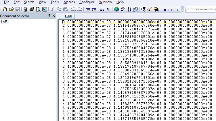
This postprocessing definition results in this file Ldiff:
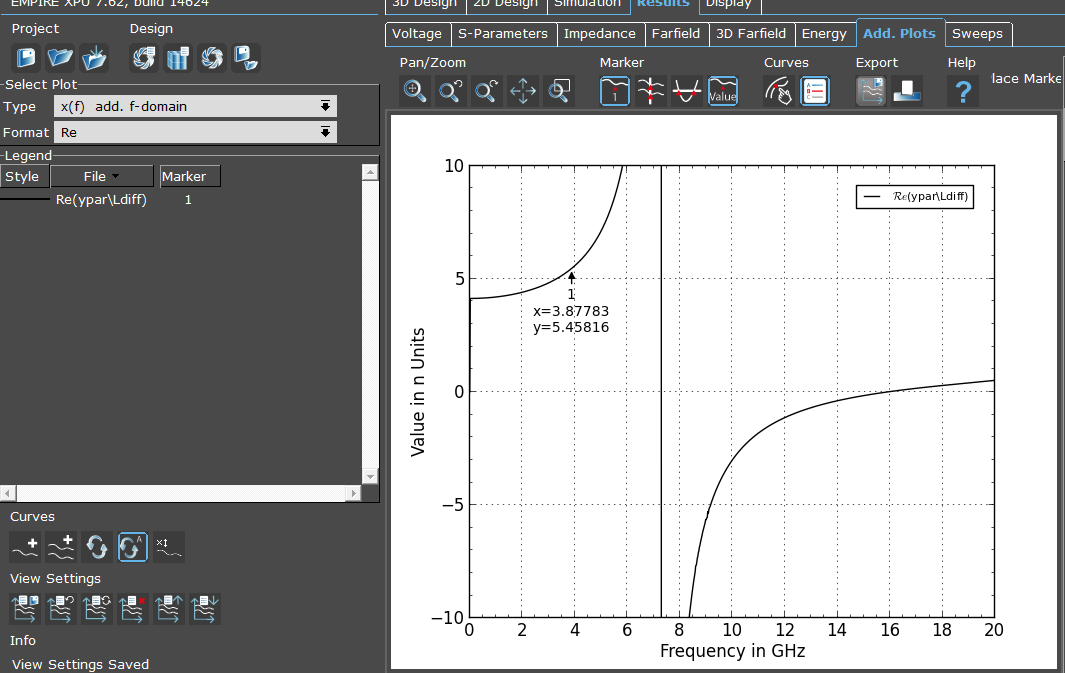
This data can now be plotted, by using the “Add. Plots” tab and selecting “x(f) add. f-domain” which means additional frequency-domain results. The file is added using the “Add data file” icon on the lower left.
Note: Inductance value is stored in real part of this data file. The imaginary part has no useful information, it’s just the zeros we defined in the previous step when using function complex (… , 0).
To use your equations in another project, you can open both projects side by side, and then use the Copy and Paste buttons in the equations tab. It is recommened to place all these custom equations into the ypar folder, because our calculation is based on Y/Z-parameter files.
That ends our tutorial. You can download the Empire example project here.

